While Rushton (1999) demonstrates, using PCA, that g and black-white differences were related, with Flynn Effect (FE) gains over time showing no relationship with the aforementioned variables, Flynn (2000) has challenged Rushton in arguing that Wechsler’s subtest loadings on the Raven test, an universally recognized measure of fluid g, showed positive correlations with both black-white differences and FE gains. Up to now, Flynn’s estimates of g fluid (Gf) has not been scrutinized. I will show presently that the Flynn’s g-fluid (call it, fluid reasoning) and Rushton’s g-crystallized (call it, consolidated knowledge) anomaly was solely due to a single statistical artifact, namely, g_Fluid vector unreliability. By adding additional samples, I created a new, updated Wechsler’s subtest Gf loadings. The present analysis comes to the conclusion that g_Fluid was not in fact correlated with FE gains. Furthermore, this Gf variable has been correlated with other variables as well, such as, heritability (h2), shared environment (c2), nonshared environment (e2), adoption IQ gains, inbreeding depression (ID), and mental retardation (MR). I will also discuss these findings in light of Kan’s (2011) thesis against the hereditarian hypothesis.
1. Introduction
The dichotomy between g crystallized (considered as depending more on prior acquired knowledge) and g fluid (as fluid reasoning, less dependent on scholastic knowledge) has not been widely considered in the many tests of Spearman’s hypothesis. In replying to Rushton, the reason why Flynn focused on g fluid is that because Flynn (2000, pp. 206-207) believes that the traditionally used g-loadings in the Wechsler are biased favorably towards more crystallized tests (the reason why he labelled the traditional g-loadings as “Gc” or g crystallized as opposed to “Gf” or g fluid). The same argument has been made by Ashton & Lee (2005). When Flynn argues that “ranking the WISC subtests in terms of fluid g would change the correlations from negative to positive” this depends on the Gc and Gf correlations. Flynn obtained a different result using his g-fluid loadings simply because Gc*Gf correlation tends toward zero. Rushton & Jensen (2010, pp. 12-14) noted this striking feature before. Additionally, Must (2003, p. 470) rightly pointed out that the dichotomy between g fluid and g crystallized is superfluous to the extent that the g-loadings of the ASVAB subtests, a highly crystallized-type test battery, correlate substantially with reaction time measures, a prototypical measure of fluid intelligence. The more complex the reaction time (RT) measures, the higher the correlation with the ASVAB g-factor (Vernon & Jensen, 1984). So, this would appear as if the more crystallized tests were also the more fluid tests at the same time. More striking is that Jensen (1998, p. 124) argued that Gf and Gc are about equally heritable, as Flynn agreed. But see Davies et al. (2009) for evidence of Gf higher heritability. Anyway, Flynn’s result is not necessarily more valid than Rushton’s. On the other hand, this tells us nothing about this controversy.
As a technical note, Flynn (2000, p. 207) explained that the correlation between Wechsler subtests with Raven matrices can be seen as an index of g_Fluid (Gf) loadings. Jensen (1980, p. 632, 1998, p. 38) indeed sees the Raven as a marker test for Spearman’s g. Besides, it is widely recognized that fluid test is less culturally influenced than crystallized test, a reason why Jensen argued that fluid-type tests like the Raven that “measures virtually nothing other than relation eduction” can be seen as the purest form of Spearman’s g. It was because FE gain was so large on fluid-type tests that Flynn has investigated this relationship. The likely reason is the increasing test-familiarity favoring gains on fluid-type tests (Kaufman, 2010a, 2010b) tending to inflate scores in recent cohorts. The huge Raven’s gains, for example, violate measurement equivalent, suggesting that the difficulty parameters of these tests are altered over time (Fox & Mitchum, 2012).
Flynn argued that Rushton’s method must be revised on the grounds that “Rushton entered five data sets for IQ gains over time, that is, data for each period and each nation. As Jensen (1998, p. 30) points out, this is a mistake: multiple data sets for a single variable are likely to have more in common with one another than they do with anything else; therefore, the factor analysis will be biased towards isolating them as a separate cluster.” (p. 212). This sounded interesting but I have to disagree. If the variables have different clustering this is because they have different pattern of correlations. I used my own data set (go to Method section) to test it, putting altogether my 5 black-white differences vectors, my 4 crystallized g, 2 fluid g, as well as inbreeding depression, and 4 Flynn effects (throwing out the Scotland sample due to missing values). Because I have used the “Dimension Reduction” SPSS procedure, there was obviously a missing value (i.e., Digit Span) from the intercorrelation. Still, the clustering was consistent with Rushton’s. After reducing the variables to the strict minimum, following Flynn’s recommendations, my correlation matrix (see Appendix) shows the same pattern of clustering.


There is no evidence that the multiplicity of variables tends to isolate different variables as separate clusters. Concerning BW-WISC difference, it was just the opposite. A possible reason is that German and Austria gains had some modest correlations with BW differences. Using FE averaged gain tends to favor a separate clustering of BW and FE because the FE averaged gain has a very low correlation with BW. Multiple data sets do not appear to affect the clustering of the variables. Instead, the clustering of any given variable was depending on the pattern of the correlations shared with all other variables. The reason Flynn’s PCA and Rushton’s PCA diverge so widely is solely due to his g_Fluid variable, which correlates substantially with FE gains and BW gap while correlating moderately with inbreeding depression.
2. Method
Data :
Flynn contra Rushton on PCA : A failed replication (EXCEL)
All the computations have been summarized in the above XLS. Only BW differences, g-loadings, heritability, shared and nonshared environment have been corrected for subtests’ differing reliabilities. Of particular importance, it must be recalled that when mental retardation (MR) has negative sign in its correlation, this means that its depressive effects are in fact related with the said variable (e.g., g-loadings). So, for example, when entering MR variables in a factor analysis, all the signs, negative and positive, need to be reversed.
To briefly introduce, I have localized three samples having Wechsler (WAIS) subtests’ correlations with Raven matrices : Vernon (1983), Rijsdijk (2002), Johnson & Bouchard (2011). This is all I found. The total N was 420, compared to the total N of 483 for Flynn’s samples (N=5) which involve exclusively WISC subtests. My final g_Fluid variable is obtained by averaging gf-WISC and gf-WAIS columns. This should improve the accuracy of estimates, as shown by its highest correlations with all other Gf column vectors.
Now, as a test of the robustness of a correlation, a method that can be employed is to simply repeat the process of removing one subtest from the column vector to see how the correlation behaves. Sometimes a near-zero correlation may become very high, sometimes a high correlation tends toward zero, and sometimes (rarely in fact) the sign of the correlation is totally reversed. This should occur more often when the subtest number is low.
Generally, PCA and MCV tests share the same shortcomings such as subtest number and vector reliability issues. My best estimates of g_Fluid vector reliability is 0.566, intentionally upwardly biased, which is much lower than g vector reliability of about 0.86 (Jensen, 1998, p. 383). As I said so many times in my previous posts, vector reliability is an artifact that must not be ignored. I will repeat here once again. Low reliability can decide both the sign and magnitude of the correlations. This is more likely to occur when the subtest number is low. Flynn, on the other hand, never considered this issue although he seems to acknowledge that he wasn’t very confident on his results. At the same time, he didn’t see PCA as an appropriate test beyond what it is aimed to do. Flynn (2000, p. 214) was right on this account :
We could then state a strong conclusion: the method of taking x in conjunction with y and z, y and z known to be genetically influenced, and then showing they all have something in common, is simply bankrupt – as a method of diagnosing whether x is genetically influenced.
This is precisely why Kan et al. (2011, pp. 51, 82-83) were skeptical about the method of correlated vectors (MCV) and principal component analysis (PCA). Indeed, structural equation modeling (SEM) analyses do a much better job in demonstrating the genetic origins of racial differences (Rowe & Cleveland, 1996; Jensen, 1998, pp. 465, 467).
3. Results
To begin, I have to say that I have computed some new variables especially for h2 and c2, due to their low reliabilities, by averaging WAIS and WISC estimates. What happens generally is that they show higher correlations with nearly all other variables probably because the ‘averaging method’ tends to enhance reliability. When h2 or c2 is mentioned below, it means I used the WAIS/WISC average.
For estimates, h2 reliability, as I computed, is about 0.628 or 0.548 with and without including the column averages, respectively. They are upwardly biased because I intentionally left aside the near-zero reliabilities. c2 reliability, as I computed, is about 0.480 or 0.436 with and without including the column averages, respectively. c2 reliability might not be so low at first glance but this is only because there was a ton of near-zero and negative reliabilities I had to ignore if we want to avoid over-correction.
Concerning regression analyses, as one would see below, some results appear clearly ambiguous. They must be interpreted very carefully (e.g., two things must be kept in mind, such as, low vector reliability of some variables and low subtest numbers).
3a. Correlational analyses
G-fluid versus G-crystallized. To begin, recall that WISC-Gf (using Flynn’s collection) and g-loadings correlated at zero. My WAIS-Gf variable correlated with g-loadings at about 0.70 and 0.80. As expected, the combined WISC/WAIS Gf correlates only modestly/acceptably with g-loadings (around 0.37-0.50). This pattern is curious considering Flynn’s comment on g-crystallization bias in the Wechsler’s test battery. Still, our result shows the following : when a subtest tends to be more crystallized it also tended to be more fluid. Because g_Fluid correlates with g-loadings, and that the more crystallized Wechsler subtests generally have the highest g-loadings, it follows that what Kan (2011) considered as being the more culture loaded tests were also the less culture loaded tests.
Subtests’ cultural loadings. Following Georgas et al. (2003), Kan (2011, pp. 41-46, 55-60) constructed a cultural loading column vector for the Wechsler subtests as well as a large variety of cognitive tests. He found that g was correlated with cultural loadings and both of them in turn correlated with subtests’ heritability and subtest black-white differences. It is surprising, still, that Kan’s cultural loading showed a Spearman correlation with g-loadings which was near-unity. Therefore we should expect g and cultural load to have the same magnitude of correlation with all other variables. Back to the present analysis, it has been found that WISC_Gf is not correlated with culture load. But WAIS_Gf correlates substantially culture load. The combined WISC/WAIS Gf showed modest/acceptable correlation with culture load. What was unexpected, as I have pointed out previously, is that culture load is not correlated with shared (c2), nonshared environment (e2) or adoption gains, while its relationship with shared environment (c2). It was also highly correlated with inbreeding depression and negatively with mental retardation (MR). Generally, culture load mimics almost perfectly heritable-g variables.
Black-white differences. A finding of interest is definitely the correlation between g_Fluid and BW difference (WISC and WAIS). The correlations lie around 0.70 and 0.80, higher than g*BW correlations. Even meta-analytic studies (Hu, Sept.21.2013; Dragt, 2010) show that g*BW correlation is about 0.70, 0.80 or 0.90 (depending somewhat on the IQ batteries) after correcting for statistical artifacts known as moderating the correlations, such as vector reliability of the two vectors, range restriction of g-loadings and deviation from perfect construct validity. But because g_Fluid reliability is lower than g, the Gf*BW must be much higher than g*BW. One would wonder however why we should give some weights on these results because of the variable’s low reliability. The reason is that when looking at my data, I noticed that all of the individual samples (N=8) showed substantial positive Gf*BW correlations. None of them were negative or tending towards zero. Therefore, while acknowledging Gf poor reliability, we can be certain that the sign of the correlation between Gf and black-white difference is really a positive one, thus rendering the artifact corrections justifiable. So then, as an example, if I correct solely for Gf reliability, it is obvious that the true correlation with BW would be near unity; taken 0.75 as an average we obtain 0.75/SQRT(0.566) = 0.997. If the correlation exceeds one, anyway, this should be interpreted as to say that the true correlation is perfect, i.e., unity.
This is important because according to Kees-Jan Kan (2011) the black-white difference is larger in the more culture loaded subtests although evidence on the contrary had been summarized by Jensen (1973, pp. 297-312; 1980, pp. 520-533, 546-575; 1998, pp. 363-365, 370). But Kan acknowledged himself, like others (e.g., Jensen, Flynn, …) that g fluid is less amenable to cultural influences than is g crystallized and, besides, Rindermann & Neubauer (2001) study suggests so. To substantiate his argument, Kan (2011) derived a cultural (or informational) loading column vector to be correlated with other variables of interest (e.g., g-loading, BW, h2, and so forth). As I have shown in my previous post, g*culture_load correlation is near unity when using Spearman rho. The Pearson correlation is about 0.80. By way of comparison, WISC g_Fluid shows no correlation with cultural load whereras WAIS g_Fluid shows a correlation of 0.581. The combined WAIS/WISC g_Fluid correlates at about 0.293 with cultural loading. Although g_Fluid reliability is much lower than g vector reliability, the g_Fluid “corrected” would still have lower correlation with cultural loading. Furthermore, when looking at Kan (2011, Table 4.1) data that were taken from Jensen (1985, Table 5) we would notice that the Raven matrices exhibit the highest black-white difference as well as the highest g-loadings when comparing it with all of the 13 WISC-R subtests. Among the 73 tests he analyzed (Table 4.1), the only cognitive tests having larger BW differences are the SAT, ACT, and ASVAB subtests. Furthermore, Fuerst (Sept.20.2013) regression analyses show that BW difference and cultural loadings correlation was in fact mediated by g. On the other hand, BW*g was not mediated by cultural loadings.
When looking at SES effects (from biological versus adoptive parents) on adoptees, the variable SES_bio shows a strong correlation with BW difference while SES_adopt is modestly correlated with BW difference. BW gap had no clear relationship with mental retardation. Respectively, BW-WISC and BW-WAIS gaps correlate modestly and strongly with h2 (about 0.29-0.21 and 0.57-0.47). Nonetheless, the h2*BW correlations look much higher with Spearman rho (0.52-0.30 and 0.77-0.67). The BW difference was not correlated with either c2 or e2 (both Pearson and Spearman).
Heritability (h2), shared (c2), nonshared (e2) environment. As detailed before, the positive correlation between g and heritability is about 0.61 (uncorrected) or 0.55 (corrected), while being negatively related with e2. Due to its low reliability, the true correlation between c2 and g is uncertain, although we note a very slight trend toward negative signs. By way of comparison, WAIS_Gf and WISC/WAIS_Gf correlate only modestly with h2 while being negatively correlated with c2 and e2. This is not to say that Gf is less heritable than is Gc, but again the observed correlation must be interpreted having in mind the low reliability of Gf. Given a g*h2 of about 0.60, vector unreliability correction would yield 0.60/SQRT(0.86*0.628) = 0.816. Comparatively, given a Gf*h2 of 0.40, the correction for vector unreliability yields 0.40/SQRT(0.566*0.628) = 0.67. But it could be argued that the greater range restriction in Gf can further attenuate this correlation relative to g*h2. But if we could simply divide the 0.072 SD of Gf by the ‘population’ SD of the Wechsler g-loadings at 0.128, thus yielding 0.56, it is obvious that Gf*h2 will easily attain 100%.
Furthermore, I correlated g_Fluid with the heritability in the 42 test batteries used in the Minnesota Twin Study data given by Johnson & Bouchard (2007, 2011) by using the Raven’s matrices correlation with the 41 remaining IQ (sub)tests to create the Gf (column) vector. So, the Gf*h2 and Gf*e2 correlations were about the same extent to that displayed by g with h2 and e2, that is, around +0.50 and -0.50, respectively. Definitely, more (very) large IQ batteries is needed to have a clearer picture on all this.
Due to the ridiculously low reliability of c2 vector, it was necessary to investigate the question of a possible Jensen effect (Gf) on c2. Thus I have correlated all the Gf individual samples with all c2 individual samples plus their averages, yielding a 11*11 matrix. The tendency is that we have more negative signs that the reverse. The positive correlations come mainly from LaBuda (1987) and Owens/Sines (1970), the latter having a very low sample size. For WAIS/WISC_c2 averaged from all of the 8 samples, the general tendency was that of a negative Jensen effect. But more samples are still needed to clarify this issue.
With regard to the secular gains, h2 as well as c2 had negative correlations with FE gains while e2 has positive correlations. My interpretation is that IQ stability is conditioned by both heritability and shared environment while IQ instability is conditioned by nonshared environment (Bishop et al., 2003; Beaver et al., 2013). Heritability also contributes to some extent to the IQ instability as well, over the course of development. With regard to mental retardation, I have summarized the results elsewhere.
Inbreeding depression. It correlates substantially with g_WISC and g_WAIS but modestly with all indices of g_Fluid and goes down to zero when using Spearman rho. But again, because our g_Fluid vector reliability is so weak, we shouldn’t focuse on this too much. The fact that Inbreeding D correlated so modestly with h2 (r=0.26, rho=0.00) is again best explained by the low reliability of, at least, h2. It also correlates with BW gap in WISC (about 0.40) but not with BW gap in WAIS; keep in mind however that BW gap in WAIS is based on only one sample (N=1880). Once again, more reliable data is needed. Inbreeding was correlated with biological parents’ SES effect on adoptees, not with adoptive parents’ SES effect on adoptees, consistent with genetic g hypothesis. It has some small correlations with FE gains, and shows a strong negative correlation with mental retardation.
Adoption gain. In Intelligence and How to Get It (2009, pp. 240-241, footnote 33) Nisbett challenged Jensen’s (1997) analysis of Capron & Duyme adoption study (1989, 1996). Inspired by Flynn’s rebuttal to Rushton PC analysis (1999), Nisbett’s expectation was that, since g_Fluid showed positive relationship with FE gains while g is negatively correlated with FE gains, the g and g_Fluid correlation with adoption (IQ) gains would have opposite signs as well. The right answer should be : “it depends”. If g and g_Fluid correlate substantially (e.g., 0.80 or 0.90) there will certainly be a high degree of chance that this can occur. But if g and g_Fluid correlation is just modest or acceptable (e.g., 0.30 or 0.50) there is no reason to expect this pattern, especially with small subtest number. Indeed, when I look at my data closely, WISC_Gf correlates at 0.400 and 0.142 with SES_bio (i.e., SES effects of biological parents on the adoptees) and SES_adopt (i.e., SES effects of adoptive parents on the adoptees), respectively. WAIS_Gf displays the same correlations, 0.694 and 0.004. The absence of g*adopt correlation may suggest the absence of Jensen effect on shared environmental influences (c2). This awaits replication.
Incidentally, SES_bio has a substantial correlation with h2 while being negatively correlated with c2 and e2. Unexpectedly, SES_adopt correlates modestly with h2, although it correlates strongly with c2 but negatively with e2, as one would expect. Also ambiguous is the fact that both SES_bio and SES_adopt correlated positively with some FE gains and negatively with some others. Both the small sample sizes of the adoption data and the modest reliability of FE gains can explain this huge variability. Finally, and as would expect g-theory, SES_bio correlated negatively with mental retardation (MR) scores while SES_adopt shows no correlation at all.
Secular gains. Flynn Effect gains were not always consistent in their correlations with other variables. For instance, FE gains in US, Germany, and Austria correlate negatively with g loadings whereas Scotland gains showed positive correlations. For the latter, we should keep in mind that Scotland had data for only 6 subtests, instead of 10 for the other Flynn effects. Having said this, some vectors of gains correlate with vectors of BW difference and some others do not. Also, some had positive correlations with WAIS/WISC Gf and some had negative correlations. A first predictable answer is obviously the method of averaging WISC and WAIS Gf, since WISC-Gf was correlated with FE gains. A second predictable answer is the modest reliability of these Flynn effects. Ignoring the Scotland sample, the FE_gain vector reliabilities are as follows : 0.459, 0.462, 0.704, 0.725, 0.536, 0.757. The mean being 0.607. Larger batteries should have higher reliabilities, thus diminishing the probability of finding outliers. In this regard, Flynn’s method of averaging all Flynn gains (into a single, unique variable) is not a bad idea but I don’t think Rushton’s choice of not having averaged the FE gains in PCA is wrong either.
Whereas WAIS/WISC Gf correlations with FE gains were inconsistent, WAIS Gf had only large negative correlations with FE. And, as said earlier, WISC Gf correlates positively with nearly all the Flynn gains except US#1 and Scotland gains. A striking feature is that secular gains correlate negatively with cultural loadings. Among the many explanations of the Flynn effect, genetic causes have to be discarded. All that remains is either cultural changes (e.g., Wicherts, 2004) or biological (Lynn, 2009). As surprising as it appears, evidence shows that biological-environmental factors’ effects are not correlated with g (Metzen, 2012). Thus if cultural change over time is the most likely explanation behind the absence of g-loadedness of FE gains, implying that cultural influences were unrelated with g as suggested by a large amount of evidence (Jensen, 1973, pp. 113-117, 1997; te Nijenhuis et al., 2007; Ritchie et al., 2013; Hu, Aug.18.2013), we are still wondering why g and cultural loadings are correlated. And especially why the latter is negatively related to Flynn Effects. See Discussion section.
3b. Regression analyses
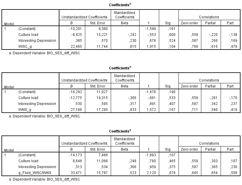
G-fluid, G-crystallized and culture load. By entering g-loadings as a dependent variable, culture load and Gf as independent variable, the expected pattern would be that culture load best predicts the g-loadings. To illustrate :

If we think using WAIS_Gf (instead of WISC/WAIS Gf) would change this figure, the picture looked the same in fact. There is no doubt that culture load partially mediates Gf*g correlation. But like I said before, the correlation between g and culture load was about 0.80 or 0.90. On the other hand, when entering Gf as dependent variable, culture load and g-loadings as independent variables, g predicts Gf while culture load had negative correlations.
If culture load is best predicting g-loadings, it wasn’t the case in Johnson/Bouchard (2011) data on 42 subtests correlations from 3 large batteries (CAB, HB, WAIS) from which intercorrelations I computed the 42 subtests’ g-loadings. Gf partially mediates culture load in the prediction of (my own estimated) g-loadings. On the other hand, when using Kan’s g-loadings as dependent variable instead, culture partially mediates Gf in predicting g-loadings (see attached XLS, sheet #1). I don’t have a clear idea about the reasons. Kan’s g-loadings and my g-loadings are poorly correlated; 0.73 seems high but it is incredibly much smaller than the usual g-loading vector reliability.

In any case, when culture and Gf (or g instead) had to predict h2, there is no mediation among the two predictors when MZA (twins) is used as estimates of h2. When Johnson et al. (2007) own estimates of genetic influences is used instead of MZA, both g anf Gf appear to (partially) mediate culture load in the prediction of h2.
Black-white differences. Fuerst noticed that BW*culture_load is mediated by g while the reverse does not stand. I confirm this. Adding to this, we can see that culture load is also (partially) mediated by inbreeding D, or by Gf, or by SES_bio in the prediction of BW difference. The picture below is self-explanatory.

When using BW-WAIS difference (instead of BW-WISC) the picture looks the same for the effect of g, Gf and SES_bio which fully mediate culture in its relationship with g. However, inbreeding D had a regression coefficient of zero, not surprising since we know that inbreeding*BW-WAIS bivariate correlation was also zero. With regard to h2, there were ambiguities because h2 fully mediates culture in the prediction of BW-WAIS gap when at the same time culture fully mediates h2 in the prediction of BW-WISC gap. In general, and perhaps due to unreliability issues, there is actually no certainty that indices of heritability mediate culture*BW correlation.
Adoption gains. Some results may appear very odd, but given the small sample size of the adoption data, we shouldn’t put too much weight on it. Now, using h2 and g (WAIS or WISC) along with culture load to predict SES_bio, I obtain the following :

These numbers are self-explanatory. g constantly had more explanatory power than h2. Culture explains nothing. Next, I use Gf instead of g to predict SES_bio. Depending on whether we use WISC or WAIS, culture load is either partially or fully mediated by the other variables, namely h2 and Gf, both of them having equal preditive power. In reality, I don’t even need to include h2. When only culture load and g are entered as independent var., g again fully mediates culture load. When I use WAIS_Gf or WAIS/WISC_Gf instead of g, the output is that culture load is only partially mediated or not at all, respectively.
In trying to replicate this result using inbreeding D instead of h2, the same picture emerges, that is, g having a strong relationship with SES_bio and inbreeding D a modest relationship with SES_bio. Similarly, when I use inbreeding D, culture load and Gf to predict SES_bio, the picture bears some resemblance except that culture has a modest positive coefficient which disappears if I use WAIS_Gf instead of WAIS/WISC_Gf.

The odd thing emerges when using SES_adopt as dependent var., with h2, culture load and g as predictors, h2 always has a strong correlation with SES_adopt, while the other variables had no relationship at all. More or less the same picture is apparent when using Gf instead of g. The only difference is that h2 has less predictive power.
Heritability and inbreeding depression. If h2 and inbreeding D are indeed correlated, it remains to be seen whether or not g will mediate this relationship, that is, if g is central in the relationship between the two indices of heritability. This appears to be the case when g and h2 are entered as independent var. with inbreeding D as dependent var., or when g and inbreeding D are entered as independent var. with h2 as the dependent var., while remembering that the correlation between g and h2 (or inbreeding D) is much stronger than the relationship between h2 and inbreeding D.
Next, I use g-fluid along with inbreeding D to predict h2 and g-fluid with h2 to predict inbreeding D. At first glance it doesn’t seem that g-fluid acts as a mediator of the relationship between h2 and inbreeding D but we had to keep in mind that the low reliability of Gf may under-estimate the importance of Gf.
When I use culture load and g-loadings to predict h2, the picture is that g*h2 correlation was partially mediated by culture load. Similarly, when using g-fluid, the contribution of g-fluid is also partially attenuated, but less. Generally, Gf constantly had more predictive power than Gc to predict h2 while controlling for culture load.

The picture is quite similar when h2, g, and culture load are entered altogether to predict inbreeding D, the g and culture load both significantly predict inbreeding D (with h2 being zero or negative) although g tends to be partially mediated by culture load. If we use Gf instead of g-loadings, Gf has weak explanatory power. Again, what would account for the difference ? To repeat, reliability of h2 and Gf is quite low and we don’t know about inbreeding D vector reliability. Nonetheless, we know that both g and culture load strongly correlate with inbreeding D and h2. But whereas cultural loadings, and not g-loadings, best predict heritability or inbreeding depression, we see that g-loadings mediate cultural loadings in predicting SES_bio.
Shared environment. As explained before, c2 had very low reliability. So, these results should be interpreted carefully. When I enter both culture and g as predictors against c2, culture now becomes strongly correlated with c2 and g stongly negatively related with c2. The picture looks similar when using Gf, but to a lesser extent. Next, when I enter c2 with g or Gf to predict BW difference (either in WISC or WAIS) c2 variable is not predicting BW differences.
Mental retardation. When entering g and inbreeding depression to predict MR, g mediates fully or partially ID*MR. One of the regression weights is outside the usual range (-1;+1). This may occur sometimes, although rarely. Anyway, when I use h2 in lieu and place of inbreeding depression, g does not mediate h2*MR and MR does not mediate g*MR. Both showed negative correlation with MR.

We have seen before that culture load correlates negatively with MR. But more often than not, when culture and g have been entered as predictors against MR, g mediates culture*MR relationship.
Regarding the indices of heritability, while h2 and inbreeding D correlate negatively with mental retardation (WISC, WISC-R, WAIS, WAIS-R), g appears to mediate inbreeding D (but not h2) in the prediction of MR. Both h2 and g have negative regression weights although h2 has a tendency to partially mediate g in WISC and WISC-R. In the WAIS, h2 fully mediates g. But in WAIS-R, there is no clear mediation and both significantly predict lower score among mental retarded people. Using Gf instead of g will be useless. WISC_Gf had positive correlation with MR, WAIS_Gf negative correlation, and WISC/WAIS a correlation of zero. Again, low reliability poses a problem for such analyses.
4. Discussion
Concerning the above findings, some variables (e.g., MR, inbreeding depression, SES_bio and SES_adopt, and FE gains) had missing values, that is, one subtest was missing (generally it was Digit Span). Thus, when partial correlation or regression analyses were applied, the bivariate correlation column (available option in regression analyses) differing somewhat from the normal bivariate correlation, the output is based on a listwise procedure.
Overall, I am not fully satisfied with regression analyses due to the difficulty of interpreting the output when using some unreliable variables and data based on small samples. And not mentioned the missing values in some variables. Adding to this, I am not satisfied either with the culture load variable. I am much more confident in that g was mediating inbreeding D and h2 than culture load mediating both g and h2 on their relationship with inbreeding D owing to my doubts about the construction of the culture load variable. That variable behaves as if it was some sort of heritable-g index rather than a generalized cultural factor as it is supposed to approximate. The absence of any relationship with environmental indices such as FE gains, adoption gains, e2 (and perhaps c2) substantiates my point. That culture load correlates both with Gc and Gf could mean either than culture load variable is not well constructed or, rather, that Gc and Gf are indistinguishable. If that is the case, the inescapable conclusion would be that Kan’s separation of g-crystallized from g-fluid, a dichotomy that Flynn has considered before, is highly misleading. And thus not justified.
Remembering what is said in the Introduction section, it seems likely that Flynn’s WISC g-fluid is anomalous and that WAIS g-fluid can be even more accurate than is the combined WAIS/WISC g-fluid. As noted before, g-loadings in crystallized biased IQ batteries tended to be correlated with measures of fluid intelligence, let alone the fact that Raven’s Progressive Matrices often exhibit the highest g-loadings when factor analyzed along with a variety of other tests, even the supposed crystallized-biased Wechsler (Jensen, 1985, p. 227, 1998, pp. 38, 120, 126-127; Vernon, 1983, Table 7; Rijsdijk, 2002). Having factor analyzed Rijsdijk (2002) and Johnson & Bouchard (2011) correlation matrices myself, there is no doubt that Raven has a relatively high g-loading to about the same extent as the Verbal IQ (VIQ) subtests and much higher than Performance IQ (PIQ) subtests. Performing another MCV test, using again Johnson & Bouchard (2007, 2011) wide test battery, the 41 (remaining) subtests’ correlations with Raven correlate with Kan’s culture load (#1 and #2) hierarchies at about the same magnitude it correlates with g which in turn is also correlated with culture load to the same extent. Overall, the problem with Kan’s expectation that culture load will track g-loadings is that the evidence for higher g-loadings in favor of crystallized over non-crystallized subtests when analyzing several large and diverse batteries is not well-established (Marshalek et al., 1983; Ashton & Lee, 2006).
Now back to the topic of the Flynn Effect, I indeed failed to replicate Flynn (2000). It is not because Flynn’s method was wrong or something. What is unfortunate is that Flynn never reported g_Fluid vector reliability. Knowing this would have greatly helped us understanding what was going wrong because among Must (2003), Rushton (2010) and te Nijenhuis (2012) who have commented Flynn’s paper, no one gave me the impression that they understood what was happening. I come to understand the Flynn/Rushton anomaly simply because I have computed the reliabilities. So then, while I was unable to replicate Flynn’s (2000) rebuttal to Rushton study (1999) I don’t believe my result is definitive. But it is surely more accurate than Flynn’s numbers due to the inclusion of additional samples.
Appendix
MATRIX DATA VARIABLES=g_Fluid_WAIS_WISC_AVG Inbreeding_Depression_WISC BW_WISC Flynn_Effect_WISC_AVG
/contents=corr
/N=5000.
BEGIN DATA.
1
0.227 1
0.715 0.476 1
0.028 0.175 0.128 1
END DATA.
EXECUTE.
FACTOR MATRIX=IN(COR=*)
/MISSING LISTWISE
/PRINT UNIVARIATE INITIAL CORRELATION SIG DET KMO EXTRACTION
/PLOT EIGEN
/CRITERIA MINEIGEN(1) ITERATE(25)
/EXTRACTION PC
/ROTATION NOROTATE
/METHOD=CORRELATION.
